Table of Contents

1. What is CFR: 3
2. Importance of CFR in a 5G transmit chain.. 4
3. Block Diagram of SoulRA CFR.. 5
4. CFR Cordic.. 9
5. CFR Matlab Simulation.. 17
6. CFR Verilog Simulation.. 18
7. CFR and BER.. 18
8. CFR optional features. 20
9. Support 20

Section 1

What is CFR:

Crest Factor reduction block minimizes the likelihood that a transmission side Power Amplifier (PA) gets saturated while transmitting a OFDM signal common in 5G. This can occur when a OFDM waveform has a high Peak to Average Power Ratio (PAPR).

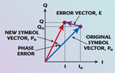
The CFR block needs to sense the maximum peak on a Symbol and reduce the maximum without altering the phase shift. CFR transmits the same QAM symbols with corrected amplitude as long as the amplitude exceeds certain magnitude.

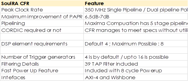
Table 1: a broad list of Features for SoulRa CFR

The first diagram illustrates the concept behind CFR to reduce the PAPR of a OFDM signal by altering I and Q without creating an error in phase.

Section 2

Importance of CFR in a 5G transmit chain

In this Section two diagrams are included the first diagram shows the location of the CFR block on the transmit side of a 5G DU.

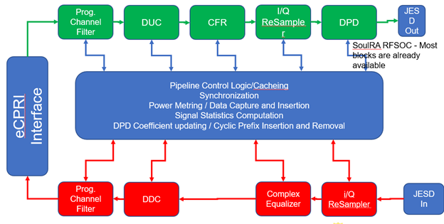
The CFR block is preceded in this diagram by a Digital Up converter and followed by a Digital

Pre-distortion block.

The second figure illustrates the 5G splits esp. the Split 7.1. The CFR is located in the Low-PHY portion of the 5G transmit chain.

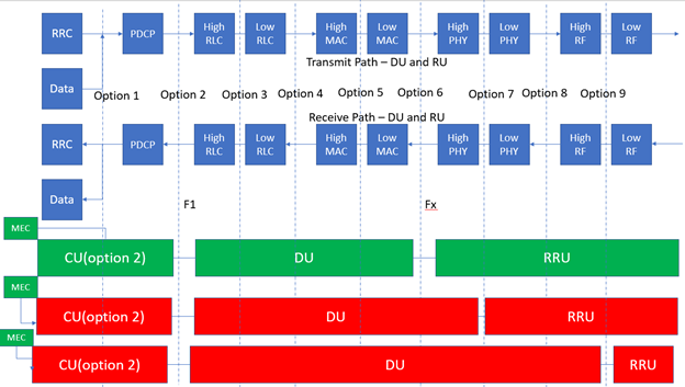
Figure 2: Complete 5G block diagram illustrating the various sub blocks

Section 3

Block Diagram of SoulRA CFR  

                            

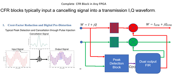
Figure 3 illustrates the CFR block. Which comprises of a peak detection sub block and a FIR filter block which is used for Peak amplitude correction without phase shifts.

The Pulse generators which can be programmed with different levels will allow the Peak to be reduced.

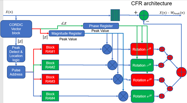
In Figure 4 the input are I and Q from I and Q Magnitude and Phase are computed without or with the usage of CORDIC. There are 6 stages.

The peak value acts as an index to 4 ROMs the Magnitude is passed to 4 RAMs.  Each RAM reduces the peak amplitude to a programmed level.

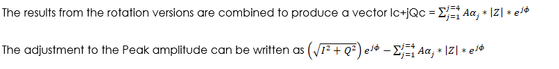
Each block RAM output is amplitude adjusted – the Peak Value multiplied by the ROM outputs.

The CFR block is designed to reduce the computational complexity

Magnitude Computation without CORDIC

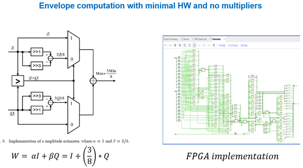
One CFR option that is provided in SoulRA IP is the magnitude computation without CORDIC. This tends to save around 400 LUT4s and some dynamic power.

The next figure provides the actual CFR implementation block with two CORDIC blocks the CORDIC block first – vectoring block and rotation block. The Vectoring block converts I and Q values into Magnitude and Phase, after operations are performed the Vectoring block transforms Magnitude and Phase into I and Q values.

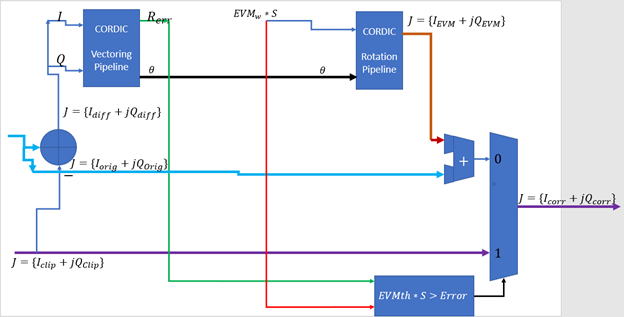
Figure 6 is the SoulRA CFR with EVM correction. It comprises of two stages – in the first stage incoming I and Q are converted into Magnitude and Phase (rectangular to Polar conversion). Also, in the first stage a difference signal between the original signal a clipped version is generated.

A simpler version of the SoulRA CFR is not EVM sensitive it just performs a Polar correction without using EVM inputs. Here is its block diagram.

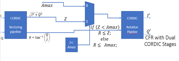
Figure 7 has two CORDIC blocks. The first block converts I, Q into magnitude and

Section 4

CFR Cordic

CORDIC block description for CFR

1 The numbers

This section describes the mathematics behind the CORDIC algorithm.

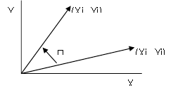
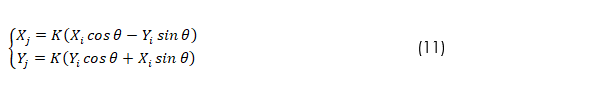
The CORDIC algorithm performs a planar rotation of a single vector over a bounded angle. Graphically, planar rotation means transforming a vector (Xi, Yi) into a new vector (Xj, Yj).

Figure 8 : Simple Rotation performed by CORDIC

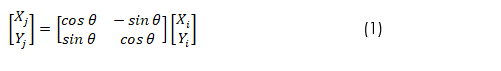
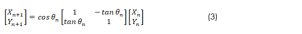
Using a matrix form, a planar rotation for a vector of (Xi, Yi) is defined as

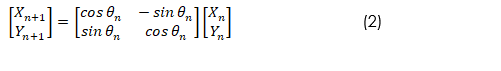
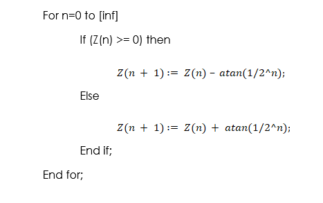
The  angle rotation is executed in multiple steps, using an iterative process. Each step completes a small part of the rotation. Many steps will be performed to compose a single planar rotation. A single step is defined by the following equation:

Equation 3 requires three multiplies, compared to the four needed in equation 2. Ultimately two of the multiplications are eliminated which is a key characteristic of CORDIC.

Additional multipliers can be eliminated by selecting the angle steps such that the tangent of a single step is a power of 2. Tangent operations are replaced with Multiplying or dividing by a power of 2 , so that it can be implemented using a simple shift operation.

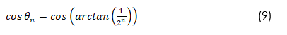
The angle for each step is given by

All iteration-angles summed must equal the rotation angle .

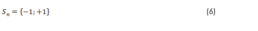
The rotation angle can be decomposed into N sub angles.

where

Combining equation 3 and 7 results in

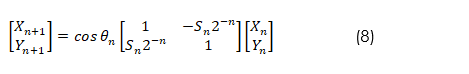
(Added) With equation 9 now step rotation step is now of fixed magnitude and the sign of thetan determines the direction of rotation – clockwise or counter-clockwise.

The second step is to compute equation 9 for all values of ‘n’ and multiplying the results, which we will refer to as K.

         

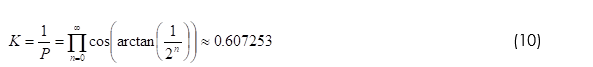
K is constant for all initial vectors and for all values of the rotation angle, it is normally referred to as the congregate constant. The derivative P (approx. 1.64676) is defined here because it is also commonly used.

We can now formulate the exact calculation the CORDIC performs

CORDIC performs the iterative set of computations for rotation with a scaling factor K

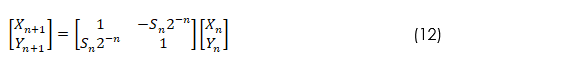
Coefficient K is pre-computed and accounted for at the final stage, equation 8 may be written as

As a 2×2 matrix computation of adding and shifting.

or expressed as two equations

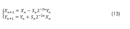
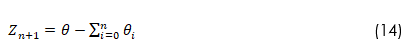
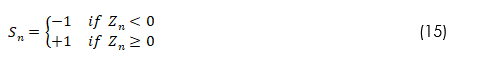
For every step of the rotation Sn is computed as a sign of Zn.

 

          

                       

                       

                       

           

Architecture

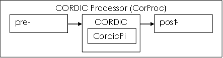
All CORDIC Processor cores are built around three fundamental blocks. The pre-processor, the post-processor and the actual CORDIC pipeline. The CORDIC core is built using a pipeline of CordicPipe blocks. Each CordicPipe block represents a single step in the iteration processes.

Figure 9:     CORDIC Processor pipeline

2.1 Pre- and Post-Processors

Because of the arctan table used in the CORDIC algorithm, it only converges in the range of –1(rad) to +1(rad). To use the CORDIC algorithm over the entire  range the inputs need to be manipulated to fit in the –1 to +1 rad. range. This is handled by the pre-processor. The post-processor corrects this and places the CORDIC core’s results in the correct quadrant. It also contains logic to correct the P-factor.

2.2 CORDIC

The CORDIC core is the heart of the CORDIC Processor Core. It performs the actual CORDIC algorithm. All iterations are performed using a fixed stage pipelined structure. Because of the pipelined structure the core can perform a CORDIC transformation each clock cycle thus ensuring the highest possible throughput.

2.3 CORDIC Pipeline

Each pipe or iteration step is performed by the CordicPipe core. It contains the atan table for each iteration and the logic needed to manipulate the X, Y and Z values.

Polar to Rectangular Conversion

The second stage of CFR performs a Polar to rectangular conversion.

After the amplitude is adjusted downwards the R and Phi values is converted using a 15 stage CORDIC pipeline into I and Q values – internal depth = 32 bits.

The rectangular to polar coordinate processor is built around the second CORDIC scheme which calculates:

5.1 Core structure

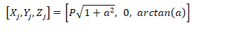
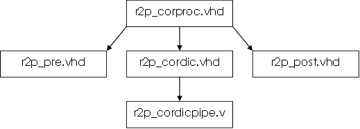
Figure 10 : File Structure  5.2 IO Ports

	Width	Direction	Description
fpgaclk	1	Input	System Clock
ENA	1	Input	Clock enable signal
Xin	16	Input	X-coordinate input. Signed value
Yin	16	Input	Y-coordinate input. Signed value
Rout	20	Output	Radius output. Unsigned value.
Aout	20	Output	Angle () output. Singed/Unsigned value.

Table 2: List of IO Ports for Rectangular to Polar CORDIC Core

The outputs are in a fractional format. The upper 16bits represent the decimal value and the lower 4bits represent the fractional value.

The angle output can be used signed and unsigned, because it represents a circle; a -180⁰ angle equals a +180⁰ angle, and a –45⁰ angle equals a +315^o angle.

CORDIC IP in Lattice Certus NX Pro FPGA LUT count Table:

Table 3: CFR FPGA resources Post Map

LUT4	PFU Registers	IO ports in IP	Carry Chain
22011	1557	104	0

Section 5

CFR Matlab Simulation

Section 6

CFR Verilog Simulation

Provided after signature of Contract

Section 7

CFR and BER

Figure 13 illustrates the concept of EVM as its applies to 5G transmitters with QAM modulation. EVM is the difference vector from the ideal constellation point to the actual constellation point.

The Difference may be due to noise or a combination of noise and nonlinearity in the system. The CFR block must consider constellation type during transmission.

The BER is a function of the EVM and EVEM is a function of the QAM-  order. Greater the number of constellation points greater can be the effect on EVM and BER. Usually at high higher EVMs the BER will be degraded.

EVM calculation formula:

The EVM is a Euclidian distance measure of the constellation points from the ideal centres of the constellation. The denominator is a Euclidean Magnitude measure of the centres of all the constellation points. The size of the sum is the QAM order N= 16,64,256,512,1024. The EVM equation is a ratio of magnitudes of noise over the magnitude of the QAM constellation points.  

Bit Error rate for M= 16/64/256 Square constellations:

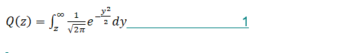
The error rate involves a Q function also known as a Gaussian Co error function which is written as

For RMS EVM the expressions can be simplified. Into a white noise expression for the numerator and a Power term in the denominator

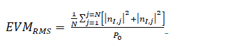
The numerator of EVM is a second order noise function. The denominator is an RMS Power expression.

Section 8

CFR optional features

Table 4

Interfaces	AXI-4 and Wishbone – other interfaces are provided extra
Matlab models	Provided for QAM rectangular

Section 9

Support

            Email: tim@soulra.net

            Email2: spondo n@soulra.net